How to adjust a DSLR Sensor after Astro Modification
The usual method to adjust a spring mounted sensor after removal and re-installation in the camera is to mark the original position of the screws and to count the turns needed to screw them in all the way down.
This is not very accurate and can go wrong if an error is made when marking the positions or counting the turns.
The only other method I have come across is based on a mechanical precision measurement, which I don't have the resources to do. So I thought of something that is easier to do.
For the solution I found you need a laser pointer, a piece of glass and - this is the most complicated part - a reasonably stable setup for it. My method compares the reflections of a laser beam on the sensor and on a piece of glass that is placed on the camera's bayonet.
The first part of the adjustment is to modify the tilt of the sensor so that the two reflected beams coincide as precisely as possible. You can even check whether an LPF1 filter that remains in the camera is correctly positioned, because that produces its own reflection that should hit the others as much as possible.
The simplest case is to let the reflected rays fall on a wall far away and check how far apart the reflections are. A more practical option is a small screen with a hole in the center through which the laser beam hits the sensor, as sketched here:
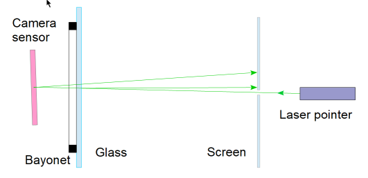
Only the most important reflections are outlined here. In fact, you get one from the front and one from the back side of the glass, but they coincide with perpendicular irradiation. The same is true for the LFP1 and LPF2 filters. From the sensor, you get two reflections from the cover glass and one from its surface.
A warning about the laser pointer: In my experience, the ones that you can buy very cheaply directly from China work well, but they sometimes produce significantly more power than is good for our eyes. So caution is definitely advised when handling such parts!
Angle adjustment
This is a reflection image from an unmodified camera at a projection distance of about four meters:
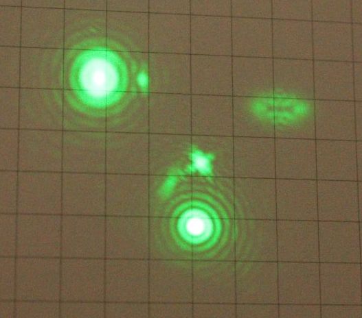
The brightest spot on the upper left comes from the glass put on the bayonet, the lower one from the sensor, and the third brightest from the filters. You can see that the factory adjustment is not quite perfect either, at least on cameras that have been in use for a while. (If you want to calculate the tilt: The grid in the picture is 5 mm wide, the distance to the camera is 4300 mm).
It is important to adjust the reflected beems as close as possible to the direction of the incident beam, because a deviation in the direction creates an additional offset.
It is important to adjust the reflected beems as close as possible to the direction of the incident beam, because a deviation in the direction creates an additional offset.
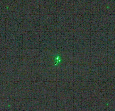
Reflections (from a second camera) on a screen in front of the laser, which shines through the hole in the middle.
The task now is to tilt the sensor so that the two main reflections coincide as precisely as possible, after the camera has been aligned so that the glass reflection, which is the brightest, falls through the hole back into the laser.
This makes the most important thing for astro applications, the angle adjustment, easy and without great effort. The exact distance of the sensor to the telescope or lens is only important if the autofocus function is required outside of live view. A defined distance is also required for a correction element (coma corrector), but it is usually sufficient to unscrew the sensor screws 360 degrees from the stop position - minus, for example, 0.3 turns for compensating a removed LPF2. In my experience, it is then accurate to +/- 0.1 mm.
If it needs to be more precise, there is also a way to measure the sensor position optically and correct it accordingly:
Measuring the sensor position
To precisely adjust the sensor position, I also use the reflection on the sensor and the diffraction effect. The diffraction effect is caused by the fact that the sensor surface is not perfectly uniform, but has a regular pixel pattern that diffracts light. You can see this very nicely in the iridescent colors that a sensor shows when exposed to white light. These colors have nothing to do with the RGB matrix, but can also be observed in monochrome sensors.
A single-colored, parallel beam of light is reflected in very specific, additional directions by this effect, which can be calculated from the sensor structure.
In fact, you can see additional, faint points of light in the corners of the screen image above. If you measure their position carefully and know the distance of the screen to the bayonet, you can use this to calculate the distance of the sensor to the bayonet.
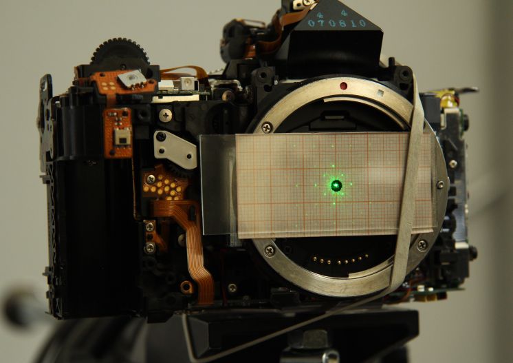
Here you can see these diffraction reflections on a special screen, which has the great advantage that its distance from the bayonet is exactly known, namely equal to zero. The position of the reflections then depends directly on the distance between the sensor and the bayonet. For the screen, graph paper is glued to a (microscope slide) glass on the camera side with clear varnish so that it becomes slightly translucent and lies directly and flatly on the bayonet.
The laser beam hits the sensor through the hole in the middle and the central reflection exits there again and returns to the laser. It is important that this main reflection falls back into the laser as precisely as possible., because then the laser beam hits the sensor perpendicularly and the formula for calculating the sensor position becomes particularly simple:
d = x · sqrt(1-y²) / y, y = m · lambda / a
with
d: (optical) distance sensor – bayonetx: distance of a reflection on the screen to the centerm: order of the reflex (1, 2, 3, ...)lambda: wavelength of the laser, 532 nm for green laser pointersa: lattice constant
The grating constant a is the size of the structures at which the light is diffracted. In the case of an RGB sensor, it is the size of an RG/GB group, i.e. twice the pixel size.
Conveniently, the distance of the sensor to the bayonet calculated in this way is immediately obtained as the optical distance, i.e. the mechanical distance reduced by the filter and cover glass effect, which is needed for the adjustment. So if you measured a distance of 44 mm before removing a filter, adjust the distance to 44 mm again afterwards.
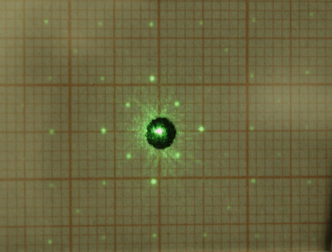
Here the diffraction pattern is shown enlarged. You can see that the reflections are on a square grid with a width of about 2.8 mm. The innermost 4 points belong to order 1, of which only the diagonal elements can be seen. Of the second order (with a center distance of about 5.6 mm in each direction), the diagonal elements are weaker than the vertical and horizontal ones, which are of zero order in one direction. This brightness distribution depends heavily on the diameter of the laser beam or on how many pixels are illuminated by the laser.
If you look at the 4th order (at 11.2 mm), you notice a kind of pincushion distortion. This means that the criteria for Fraunhofer diffraction are not sufficiently met. The equation above can therefore no longer be applied to reflections that are far out. For the points of order (4,0) on the horizontal and (0,4) on the vertical through the center however, I always got results that were as good as the reading accuracy of about 0.1 mm.
As an example, here is the calculation for order (4,0):
2 · x = 22.4 mm (4th order distance left and right of the center)
The camera is an EOS 60D with a pixel size of about 4.30 µm, so a = 8.6 µm.
This means
y = 4 · 532 nm / 8.6 µm = 0.2474 with: sqrt(1-y²) / y = 3.916 .
The distance of the sensor from the screen is:
d = x · sqrt(1-y²) / y = 11.2 mm · 3.916 = 43.86 mm
The deviation from the Canon EF flange focal distance is therefore 0.14 mm, which is about the same as the (relative) uncertainty when reading '2 · x'.
Some uncertainty in the calculation is the pixel size that can be found for the cameras. I have also found 4.29 µm for the 60D instead of the 4.3 µm, which makes also about 0.1 mm difference on the result, and 'official', exact values I could not find, unfortunately.
Another potential source of error is the graph paper, which might change its size slightly when glued on. To improve accuracy, it is therefore not a bad idea to carry out the measurement once before disassembling the camera in order to calibrate the method.
Direct measurement using the sensor
To improve the reading accuracy, I have thought of another variant, which can, however, only be used with a camera that is ready for operation. Instead of reading the diffraction reflections from graph paper, the diffraction patterns are reflected back onto the sensor. This is achieved by placing a surface mirror (with a hole in the center) on the lens mount. A simple glass will also suffice, as glass reflects light well enough for this purpose.
The diffraction pattern reflected back onto the sensor can be read out in a very high-resolution image. Furthermore, the spacing between the reflections doubles, making it easy to use first- or second-order diffraction patterns, which are practically unaffected by pincushion distortion.
This is what the light path looks like when the left side of the glass is mirrored:
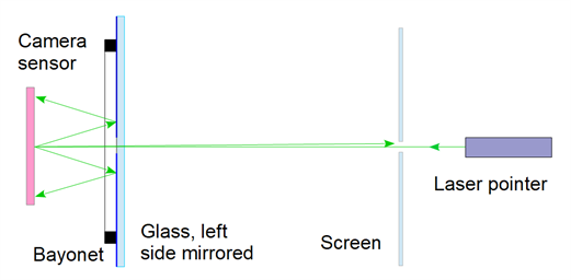
If you use uncoated glass as a mirror, the main part of the diffracted rays exits through the glass, only 4% of the intensity is reflected. From the exiting part you get an additional reflection on the outside of the glass. Double dots then appear on the sensor:
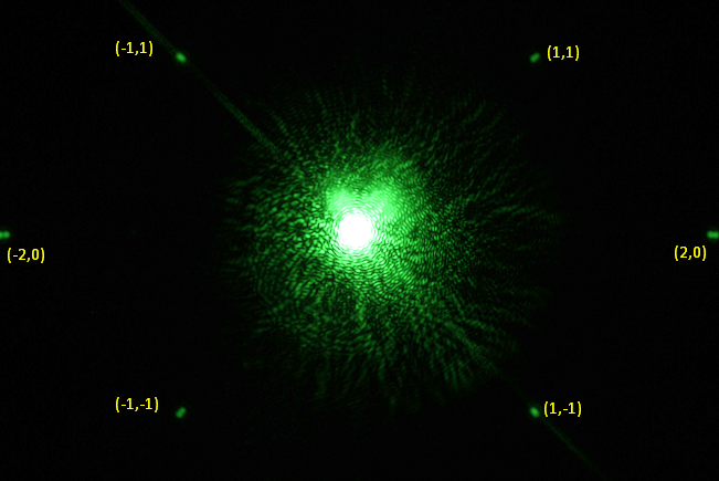
Although the exposure time for this shot was only 1/250 s, the sensor around the direct laser point is massively overexposed, which cannot be avoided if you want to see the diffraction reflections. But it is not a problem, and the low laser power cannot harm the sensor either.
The second order reflections just fit on the APSC sensor here, and it is easy to see that the diffraction reflections always consist of two points, with the outer ones coming from the outer side of the glass.
To calculate the sensor position, it is best to use the distances between the inner points and their counterparts, then it does not matter how thick the glass is.
The distance w between the (-1,-1) and the (1,-1) reflection was 2540 pixels, which again have a size of approx. 4.3 µm. Inserted, this gives (with y1 being the y for the first order)
d = w/4 · sqrt(1-y1²) / y1 = 2540/4 · 4.3 µm · 16.13 = 44.06 mm
With the (-2.0) and (2.0) reflections, d = 44.01 mm results.
The accuracy is limited here by the diameters of the reflection points. Added to this is the error in the pixel size used, which has a significantly greater impact here than above, because the pixel spacing is also factored into the measured reflection distance. And gradually, the decimal places of the laser wavelength also become relevant.
Laser
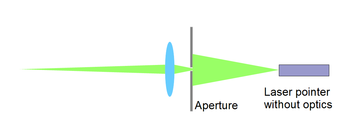
To improve the quality of the laser beam, I first widened it, then blocked out most of it with a small aperture and finally focused it so that the focus is close to the sensor. In addition to the better image, this has the advantage that I have reduced the power to less than a hundredth, which then makes a laser pointer really safe. To widen the beam, you can simply remove the built-in lens. To focus, you need a focal length that is slightly longer than half the desired distance between the lens and the laser or the sensor, e.g. f = 100 mm. (However, correcting the sensor tilt works just as well with an untuned laser.)
Inexpensive green lasers are frequency-doubled Nd:YAG lasers. For measuring the sensor position they have the advantage over diode lasers that the wavelength (532 nm) is precisely known and the beam quality cannot be too bad due to their design. Red lasers are diode lasers that come in different wavelengths. So you first have to find out whether it is 635 nm or 650 nm or some other wavelength. They have the additional disadvantage that they are greatly weakened by the LPF2 filter, so that reflections from the sensor of unmodified cameras are quite faint.
Finally, the grating equation for calculating the diffraction pattern:
The angle phi of the main maximum of order m of a diffraction grating is
sin(phi) = sin(phi0) ± m · lambda/a
where the angle of incidence phi0 is best set to 0°.
Its position x on a screen at a distance d is
x = d · tan(phi)
Both together give
d = x / tan(asin(y)) with: y = m lambda/a
or
d = x · sqrt(1-y²) / y
Last updated on January 8, 2026